Ipek Balikci Cicek^1*, Zeynep Kucukakcali²

¹Department of Biostatistics and Medical Informatics, Inonu University Faculty of Medicine, 44280, Malatya, Turkey. ORCID: 0000-0002-3805- 9214

²Department of Biostatistics and Medical Informatics, Inonu University Faculty of Medicine, 44280, Malatya, Turkey. ORCID: 0000-0001-7956- 9272

*Corresponding Author: Ipek Balikci Cicek, Department of Biostatistics and Medical Informatics, Inonu University Faculty of Medicine, 44280, Malatya, Turkey. ORCID: 0000-0002-3805-9214.

Abstract
Object: Chronic kidney disease (CKD) is a worldwide public health problem with a high morbidity and mortality rate, as well as a risk factor for other illnesses. Clinicians may miss the disease because there are no apparent signs in the early stages of CKD. Early detection of CKD helps patients to get prompt therapy to reduce disease progression. Machine learning (ML) models, with their speedy and accurate detection capabilities, can successfully assist physicians in achieving this goal. Given that ML models are considered "black boxes," it is also required to reveal the significant factors that led a model to anticipate a specific outcome. In this article, using CKD open access data, the ML model is interpreted with the Shapley Additive explanations (SHAP) explainable artificial intelligence (XAI) method, which is based on fair profit distribution depending on the contributions of many stakeholders.

Method: In this study, the open-access dataset named "Chronic Kidney Disease" includes 400 patients with and without CKD. ML classifiers are employed in this article to predict if the patient has CKD or not. In this article, four tree-based ML classifiers (decision tree, AdaBoost, XGBoost, and Random forest -RF) are used to predict whether the patient has chronic kidney disease (CKD). The RF model achieved the best performance among tree-based ML models with 99.00% prediction accuracy. The SHAP method, an explainable approach, was used for local and global explanations of the RF model's decisions. In the modeling process, the 10-fold cross-validation technique was used, and the dataset was split into 80% training and 20% testing. Datasets. The accuracy (ACC), balanced accuracy (b-ACC), specificity (SP), sensitivity (SE), negative predictive value (npv), positive predictive value (PPV), and F1-score metrics were used to evaluate the model.

Results: The RF technique of modeling yielded performance metrics for ACC, b-ACC, SE, SP, PPV, npv, and F1-score, which were 99.0%, 98.6%, 97.3%, 100%,100%, 98.4%, 98.6%, and respectively. According to the variable importance result obtained from the SHAP method, Hemo, Sg, Al, Sc, and Rbcc variables are the five most influential variables in predicting CKD/Not CKD.

Conclusion: With the current study, CKD was predicted, and the risk factors that may impact CKD were given with the SHAP model to shed light on the interpretation part that is a problem for users after modeling. With SHAP used after ML, the results are presented individually and globally. This helps clinicians intuitively understand the model results.

Keywords: Chronic kidney disease, classification, machine learning, explainable artificial intelligence, risk factor, Shapley Additive Explanations

Introduction
Chronic Kidney Disease (CKD), also known as chronic renal disease, is a long-term medical disorder in which the kidneys gradually lose their function. The kidneys filter waste and excess fluids from the circulation, ultimately expelled as urine. When the kidneys are injured or compromised, waste and fluids accumulate in the body, resulting in various issues [1]. Globally, CKD is a significant public health issue, especially in low- and middle-income nations where millions of individuals lose their lives to treatment-related complications. 14% of people globally suffer from CKD, making it a serious issue. Today, more than 2 million people need dialysis or a kidney transplant to survive, although this number may only represent 10% of those who need medical attention [2].

Two fundamental methods are used by medical professionals to gather precise patient information to identify kidney disease. Initially, testing for CKD is performed on the patient using both urine and blood. A blood test can measure the glomerular filtration rate (GFR), which measures renal function. Normal kidney function is indicated by a GFR of 60; poor renal function is indicated by values between 15 and 60. Finally, a GFR of 15 or below shows kidney failure. The second technique, urinalysis, checks for albumin, which can be seen in urine when the kidneys are not operating correctly [3]. Early detection is critical for lowering CKD mortality rates. Late diagnosis of this illness causes renal failure, necessitating dialysis or kidney transplantation [4]. The expanding number of CKD patients, along with a need for more trained physicians, has resulted in expensive diagnostic and treatment expenses. Computer-assisted diagnostic technologies, particularly in developing nations, are required to aid radiologists and doctors in diagnostic decision-making [5].

In such cases, computer-aided diagnostics can be essential in determining the disease's prognosis early and efficiently. ML methods, a subdomain of artificial intelligence (AI), may be used to identify a disease accurately. These methods are intended to help clinical decision-makers undertake more accurate illness categorization. ML is becoming more important in healthcare diagnostics because it allows for comprehensive analysis, reducing human mistakes, and increasing forecast precision. ML algorithms and classifiers are increasingly regarded as the most reliable approaches for predicting illnesses such as heart disease, diabetes, tumor disease, and liver disease [6].

The vast majority of ML models are regarded as "black boxes." A black-box model is so complex that it cannot be easily comprehended by humans [7,8]. It is difficult for clinicians to grasp what caused the black box model to anticipate a given outcome when utilizing it as a diagnostic method. From the standpoint of clinicians and patients [9,10], black box techniques impede medical decision support. As a result, it is required to create a diagnostic system that ensures the interpretability of the ML model [7,9,11]. The ML model's interpretability increases the doctors' trust in the system by providing a safety check on the expected outcomes. Research interest in the field of XAI has expanded recently to solve the ML model's interpretability [12,13].

In this article, SHAP, one of the XAI methods, was used for the interpretability of the ML model. SHAP is a prominent and frequently used ML and interpretability approach. It is intended to explain the output of ML models by attributing a specific instance's prediction to its unique attributes, hence offering insights into the model's decision-making process [14]. SHAP is based on cooperative game theory and the Shapley values idea. Shapley values assign a value to each characteristic based on how well it predicts. It computes how much each feature "contributes" to the difference in prediction between the model and the expected prediction [15].

The purpose of current research is to create an automated interpretable CKD diagnosis system that displays the priority of the variables that impacted the system's decision to diagnose CKD or not. The CKD diagnostic system, an interpretable ML model employing SHAP, and an evaluation of the attribute contribution to CKD prediction are the main contributions of this article.

The remainder of the article is organized as follows. The "Methodology" section describes the dataset, classification methods, SHAP, and performance metrics. In the Results section, the detailed results of the classification methods used and the RF classification method, and the findings we obtained from the SHAP analysis are presented respectively. Explanations about the results are made in the "Discussion" section.

Methodology
Dataset
The "Chronic Kidney Disease" open access dataset was taken from https://www.kaggle.com/abhia1999/chronic-kidneydisease. The CKD Data set contains 14 characteristics of 400 patients. Of the 400 patients, 250 (62.5%) are CKD patients and 150 (37.5%) are not CKD patients.

Table 1 lists the 14 independent variables in the CKD dataset, including 1 dependent variable and their explanations.

Table 1: Descriptions of variables included in the CKD dataset

Classifier
This part explains the ML methods we used to classify the CKD dataset. The classifiers are types of ML algorithm that categorizes input into predefined classifications. In this case, the classifier will utilize the patient's attributes as input to identify whether or not the patient has CKD.

Random Forest, Adaptive Boosting, Decision Tree, and Extreme Gradient Boosting tree-based ML methods were used to predict whether the patient had CKD.

Decision Tree (DT)
DT was first proposed by Breiman et al. [16]. Classification of data using this method is performed in two stages. The first stage is called the learning stage, and the second stage is called the test data stage. In the learning phase, a known learning data set is identified by the classification algorithm to create a model. The learned model generates classification rules and is expressed as a decision tree. The test data phase is used to assess the classification rules' correctness. If the classification rules' accuracy is adequate, the resulting rules can be utilized to categorize the new data [17].

Adaptive Boosting (AdaBoost)
AdaBoost is a Boosting technique used as an ensemble accelerator classifier in ML, proposed by Robert Schapire and Yoav Freund in 1996. The Adaboost approach works by adjusting the classifier weights and training the data sample at each iteration to offer accurate predictions of observations. The steps of the working principle of the Adaboost algorithm are as follows. First, Adaboost randomly selects a training subset. Based on the accurate prediction of the final training, it determines the training set and trains the AdaBoost ML model iteratively. Misclassified observations are assigned higher weights so that in the next iteration, these observations have a higher probability of classification. It also gives importance to the trained classifier at each step based on the accuracy of the classifier. The more accurate classifier will receive a higher weight. This process is repeated until all training data is fitted without errors or the maximum number of predictors is reached [18].

Extreme Gradient Boosting (XGBoost)
XGBoost is a supervised learning technique that uses gradient boosting machines (GBM), one of the most powerful supervised learning algorithms. GBM and DT algorithms serve as the foundation of its basic architecture. It performs and moves faster than other algorithms, which is a significant benefit. Additionally, XGBoost is ten times quicker than competing algorithms, has a high level of predictive ability, and incorporates several regularizations that enhance performance overall while lowering overfitting or overlearning. A series of weak classifiers are combined with boosting in a technique known as gradient boosting to produce a robust classifier. The strong learner is progressively trained, beginning with a primary learner. The underlying ideas behind XGBoost and gradient boosting are identical. The implementation specifics are where the main variances lie. XGBoost can improve performance by using a variety of regularization approaches while managing the complexity of the trees [19].

Random Forest
Breiman (2001) introduced the random forest approach, a machine learning algorithm combining Bagging and Random Subspaces techniques. It consists of many decision trees. The RF method combines the calculations of many decision trees to provide a conclusion. It is a supervised machine-learning technique. It is well- liked since it is straightforward but efficient. Due to its versatility and ease of use, it has often been used for solving regression and classification issues [20]. The dataset is initially randomly separated into two portions in the RF algorithm: training data for learning and validation data to assess the level of learning. Following that, the "bootstrap method" is used to build multiple decision trees at random from the dataset. Each tree's branching is governed by randomly selected determinants at node positions. The RF forecast is the average of all the tree's results.

As a consequence, each tree influences the RF prediction for specific weights. Because of its capacity to randomly accept training data from subsets and generate trees using random ways, the RF algorithm outperforms other machine learning algorithms. Furthermore, because the RF technique trains on different randomly selected subsets of data via bootstrap sampling, the amount of overfitting is maintained [21].

SHAP
SHAP is a model-agnostic game theory-inspired method that attempts to increase interpretability by calculating the importance values for each characteristic for individual predictions. For each prediction, the SHAP computes an additive feature importance score that maintains three desirable properties: missingness, consistency, and local accuracy [12]. The SHAP helps describe and illustrate how a feature value may be used to forecast using SHAP values. The SHAP values give a dynamic perspective of the effects of feature interaction in calculating risk probability and the unique importance of each attribute. Furthermore, the SHAP allows you to present and explain the qualities in charge of prediction at both the local and global levels [22].

Performance metrics
In this study, performance metrics ACC, b-ACC, SE, SP, PPV, npv, and F1 score are the measurement approaches used to measure how well the classification ML model performs. ACC has been used to measure the effectiveness of tree-based models.

Python 3.6.5 (sklearn, Decision tree, AdaBoost, Random Forest, XGBoost, and sharp packages) was used for all analyses and computations.

The data is divided into 80% training and 20% test data. To confirm model validity, the n-fold cross-validation approach, one of the resampling methods, was used in this study. In • The dataset is first divided into n pieces, and the model is then applied to those pieces. • In the second step, one of the n parts is used for testing, while the remaining n-1 parts are used for training. • Finally, the cross-validation approach is evaluated using the average values collected from the models.

The workflow diagram for the development of the dataset to be used in the study and the modeling process to be applied is given in Figure 1.

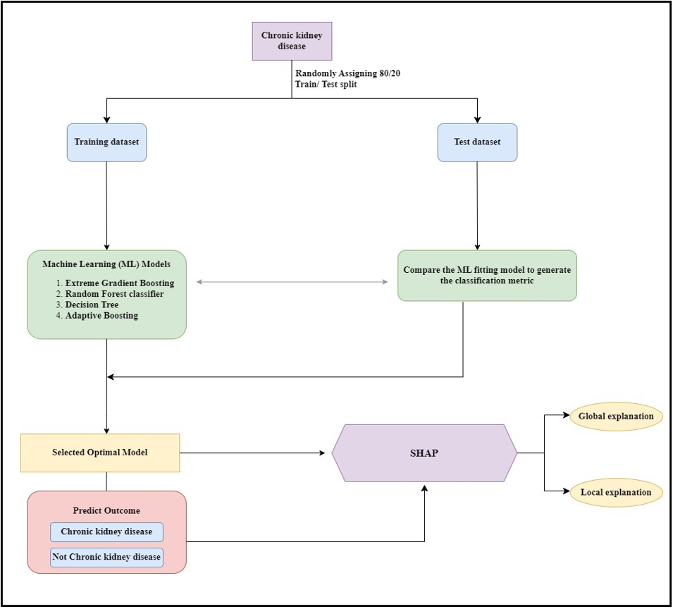
Figure 1: The workflow diagram.

Results
In this study, 4 classification models were used for training. These are XGBoost, AdaBoost, RF, and DT classification methods. The dataset was randomly split into three parts: 80% training data and 20% test data.

Table 1 shows the values of the performance measures derived by modeling with ML methods using person's CKD and not CKD.

Table 1: Performance metrics values obtained after modeling.

ML: Machine Learning; ACC: Accuracy

Among the DT, AdaBoost, XGBoost and RF ML models used in the study, the RF model showed the best performance in terms of test accuracy. The results of the performance metrics obtained from the RF model are given in Table 2.

Table 2: Performance metrics values obtained after modeling of RF

ACC: Accuracy; b-ACC: Balanced accuracy; SP: Specificity; SE: Sensitivity; npv: Negative predictive value; ppv: Positive predictive value The SHAP variable importance graph showing the effect of each variable on the target variable is given in Figure 2.

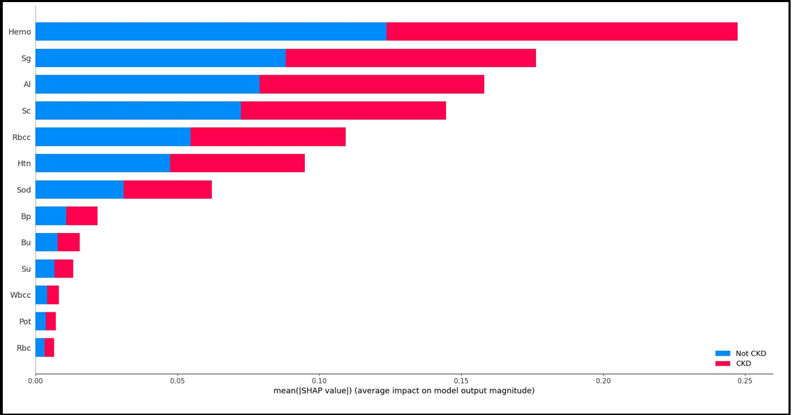
Figure 2: SHAP variable significance plot

Figure 3A and Figure 3B show the Beeswarm SHAP plots, which indicates in which direction (positive/negative) and in what proportion (magnitude/smallness) each variable is effective in explaining the target variable (CKD/not CKD). Figure 3A shows the results for the not CKD category while Figure 3B shows the results for the ckd category. When the graphs are analyzed, it is seen that the two graphs obtained are inverted in terms of direction and values when the categories change.

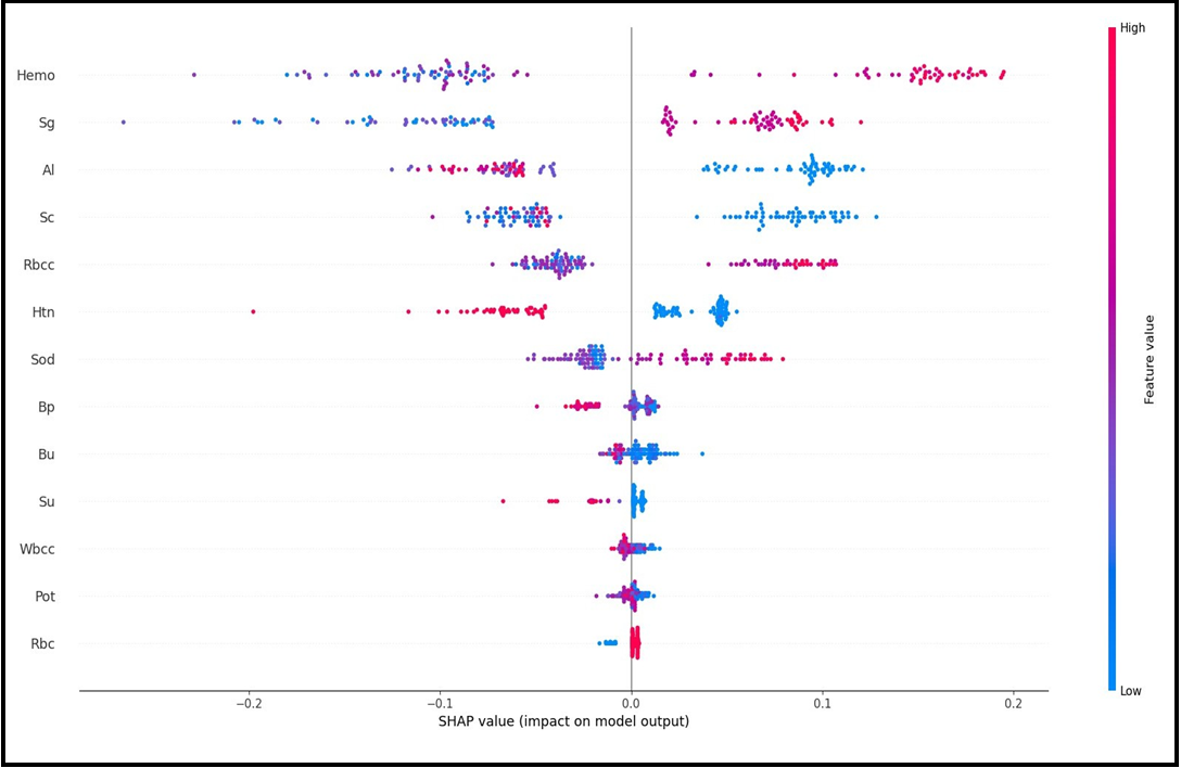
Figure 3(A) SHAP Beeswarm Plot

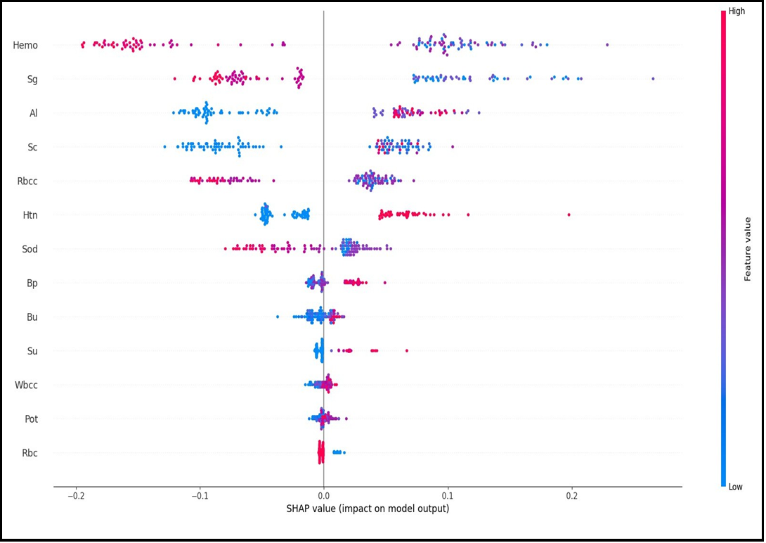
Figure 3(B) SHAP Beeswarm Plot

Figure 2, Figure 3A and Figure 3B above are graphs that can be used for global interpretation of explainable AI models and show the contributions of variables to the target variable by considering all observations. Explainable AI models also allow for individual interpretation. While some models only allow for individual interpretations, some models allow for both global and local interpretations.

Figure 4A and Figure 4B show the local interpretation results of the SHAP method that allows both interpretations. Figure 4A and Figure 4B SHAP force graphs are given. Figure 4A and Figure 4B are inverted versions of each other and present local explanations for each individual according to the categories of the target variable.

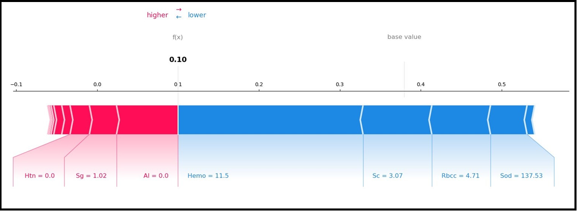
Figure 4(A) SHAP Force Plot

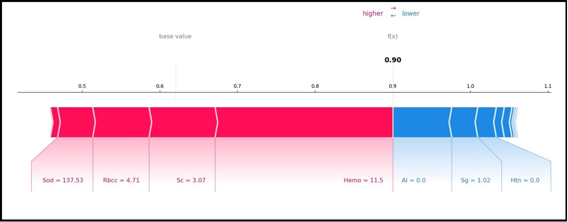
Figure 4(B) SHAP Force Plot

The SHAP method decision graphs demonstrate how total estimations vary during the decision-making process. On the Y-axis, characteristics are listed in order of contribution. The model's output is represented on the X-axis. The SHAP value of each feature is totaled for the base value of the model while going from the bottom to the top of the plot to produce the final output value, as in the SHAP summary plot. As a result, it is feasible to identify how much each characteristic contributes to the outcome throughout the total estimating process.

SHAP decision graphs are given in Figure 5A and Figure 5B. Figure 5A and Figure 5B are reversed and present local explanations for each individual according to the categories of the target variable. Figure 5A shows how much individual characteristics contribute to the model prediction of the grade as CKD. Figure 5B shows how much individual characteristics contribute to the model prediction as CKD.

Figure 5(A)

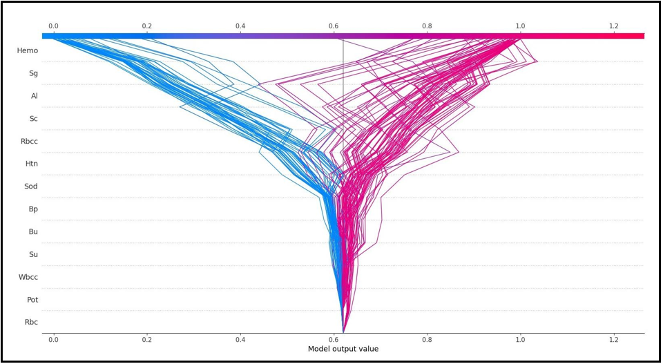
Figure 5(B)

Discussion
CKD is a kind of kidney disease in which the glomerular filtration rate (GFR) gradually declines over three months [23]. Because there are no physical indications in the early stages, it is a silent killer. In 2016, 753 million individuals worldwide were impacted by CKD [24]. Every year, over 1 million individuals in 112 impoverished countries die from renal failure because they cannot afford the high cost of frequent dialysis or kidney replacement operations. To lessen the burden of CKD on public health, early identification, and effective treatments are critical [25]. The timeline for routine health checkups varies per country due to changing economic situations. Even within the same country, various populations receive different degrees of health screening. In most nations, a complete routine health examination, especially for the diagnosis of frequent deadly illnesses such as cancer and heart disease, is uncommon. Only when there is a clinical problem are CKD tests undertaken, and by then, it is too late [26].

Early detection of CKD patients who are at a high risk of developing clinical deterioration is essential because it may help with the provision of the proper care and the economical use of the little resources available [27]. Therefore, creating predictive models that can reliably predict whether an individual is ill may aid clinical practice. ML algorithms have the potential to reduce the risk of CKD-related death in critically sick patients due to their capacity to analyze massive volumes of data from electronic health records. These may include demographic data, treatments, measures that are taken regularly, and patient diagnoses. These state-of-the-art data-driven algorithms are capable of handling high-dimensional data, evaluating intricate connections, and locating essential outcome predictors. Compared to traditional modeling approaches, which employ variables primarily selected for their statistical or clinical relevance and demand that predictors be independent of one another, they are more flexible. [28,29]. ML techniques have been widely used in illness prediction in recent years. Clinicians may more effectively screen for and identify patients at high risk of unfavorable outcomes with the help of a well-designed prediction model, enabling more prompt intervention and better results [30,31].

Furthermore, there needs to be more information regarding its usefulness in a real-world clinical setting and in explainable risk prediction models to support illness prognosis despite earlier research demonstrating encouraging outcomes [32,33]. The "black-box" nature of machine learning algorithms makes it challenging to justify the assumptions that underlie individual patient forecasts, i.e., the particular patient characteristics that contribute to a specific prognosis. One of the main obstacles to ML deployment in the medical field is the lack of an intuitive grasp of ML models, which has so far restricted the application of more potent ML techniques in medical decision support due to their lack of interpretability [34,35]. This study used an advanced machine learning algorithm with a SHAP-based architecture to overcome these drawbacks. Consequently, this study not only improved the ML model's predictive accuracy for CKD prediction, but it also offered heuristic explanations that assisted patients in anticipating risk. This made it easier for medical professionals to comprehend how to make decisions about how serious an illness is and how to increase the likelihood of early intervention.

The outputs of the SHAP graphs obtained in the current study are given in detail below. According to the SHAP variable importance graph (Figure 2), Hemo, Sg, Al, Sc, and Rbcc are the five most influential variables in predicting CKD/Not CKD (target variable). According to the Beeswarm SHAP graphs (Figure 3A, Figure 3B), since high SHAP values of Hemo and Sg variables show a negative trend, they will have a negative effect in explaining the target variable and support grade CKD. In other words, while high Hemo values are associated with grade CKD, on the contrary, low Hemo values will be related to the CKD category. In the same way, high values of the Sg variable will show a negative trend and affect the target variable in the opposite direction, and low values of the Sg variable will be associated with CKD. The relationships of the other variables in the graph with the target variable are interpreted similarly. The SHAP force plots in Figure 4A and Figure 4B show the local results of the first patient in the test data. Figure 4A explains the not CKD category, and Figure 4B for the CKD category. Figure 4B shows that Hemo=11.5, Sc=3.07, Rbcc=4.71, and Sod=137.53 of the first patient in the test data have a positive contribution to being not CKD.

On the other hand, Al=0.0, Sg=1.02, and Htn=0.0 values of the first patient in the test data have a negative contribution to CKD. In addition, the SHAP method predicted that this patient had CKD with a 90% probability. According to the findings obtained from SHAP decision graphs (Figure 5A, Figure 5B), the order of the variables that make the most significant contribution to the overall prediction is as follows: Hemo, Sg, Al, Sc, Rbcc.

The results obtained from this study support the literature. With this study, a significant step forward has been taken for ML in medicine. It will also help develop interpretable and personalized risk prediction models.

The results obtained from this study support the literature. However, there are limited studies in the literature on methods that will bring transparency to black box models that can predict CKD, that is, shed light on how and why a particular decision is made. Thus, with this study, a significant step forward has been taken for ML and XAI models in medicine by contributing to the literature on this subject. It will also help develop interpretable and personalized risk prediction models.

References

1. Gwozdzinski K, Pieniazek A, Gwozdzinski L (2021) Reactive oxygen species and their involvement in red blood cell damage in chronic kidney disease. Oxidative medicine and cellular longevity. 2021: 6639199.
2. Ekanayake U, Herath D (2020) Chronic kidney disease prediction using machine learning methods," in 2020 Moratuwa Engineering Research Conference (MERCon). 260-265.
3. Swain D, Mehta U, Bhatt A, Patel H, Patel K, et al. (2023) A Robust Chronic Kidney Disease Classifier Using Machine Learning Electronics. 12(1): 212.
4. Garcia GG, Harden P, Chapman J (2012) The global role of kidney transplantation. Archives of Iranian Medicine. 1(2): 69-76.
5. Senan EM, Al-Adhaileh MH, Alsaade FW, Aldhyani THH, Alqarni AA, et al. (2021) Diagnosis of chronic kidney disease using effective classification algorithms and recursive feature elimination techniques. Journal of Healthcare Engineering. 2021: 1004767.
6. Kavitha M, Gnaneswar G, Dinesh R, Rohith Sai Y, Sai Suraj R (2021) Heart disease prediction using hybrid machine learning model. in 2021 6th international conference on inventive computation technologies (ICICT). 1329-1333
7. Petch J, Di S, Nelson W (2022) Opening the black box: the promise and limitations of explainable machine learning in cardiology," Canadian Journal of Cardiology. 38(2): 204-213.
8. Adadi A, Berrada M (2018) Peeking inside the black-box: a survey on explainable artificial intelligence (XAI)," IEEE access. 6: 52138-52160.
9. Montavon G, Samek W, Müller KR (2018) Methods for interpreting and understanding deep neural networks. Digital signal processing. 73: 1-15.
10. Yang G, Ye Q, Xia J (2022) Unbox the black-box for the medical explainable AI via multi-modal and multi-centre data fusion: A mini-review, two showcases and beyond. Information Fusion. 77: 29-52.
11. Ahmad MA, Eckert C, Teredesai A (2018) Interpretable machine learning in healthcare. ACM international conference on bioinformatics, computational biology, and health informatics. 559-560.
12. Linardatos P, Papastefanopoulos V, Kotsiantis S (2020) Explainable ai: A review of machine learning interpretability methods. Entropy. 23: 18.
13. Tjoa E, Guan C (2020) A survey on explainable artificial intelligence (xai): Toward medical xai. IEEE transactions on neural networks and learning systems. 32: 4793-4813.
14. Lundberg S, Lee S-I (2017) A unified approach to interpreting model predictions. Advances in neural information processing systems. 30: 4768-4777.
15. Kuzlu M, Cali U, Sharma V, Güler Ö (2020) Gaining insight into solar photovoltaic power generation forecasting utilizing explainable artificial intelligence tools. IEEE Access. 8: 187814- 187823.
16. Breiman L, Friedman J, Stone CJ, Olshen RA (1984) Classification and regression trees: CRC press.
17. Somvanshi M, Chavan P, Tambade S, Shinde S (2016) A review of machine learning techniques using decision tree and support vector machine. in 2016 international conference on computing communication control and automation (ICCUBEA). 1-7.
18. Sprenger M, Schemm S, Oechslin R, Jenkner J (2017) Nowcasting foehn wind events using the adaboost machine learning algorithm," Weather and Forecasting. 32(3): 1079-1099.
19. Salam Patrous Z (2018) Evaluating XGBoost for user classification by using behavioral features extracted from smartphone sensors.
20. Asadi S, Roshan S, Kattan MW (2021) Random forest swarm optimization-based for heart diseases diagnosis," Journal of Biomedical Informatics. 115: 103690.
21. Asselman A, Khaldi M, Aammou S (2023) Enhancing the prediction of student performance based on the machine learning XGBoost algorithm. Interactive Learning Environments. 31(3): 3360-3379.
22. Belle V, Papantonis I (2021) Principles and practice of explainable machine learning. Frontiers in big Data. 4: 688969.
23. Stevens PE, Levin A (2013) Evaluation and management of chronic kidney disease: synopsis of the kidney disease: improving global outcomes 2012 clinical practice guideline. Annals of internal medicine. 158(11): 825-830.
24. Bikbov B, Perico N, Remuzzi G (2018) Disparities in chronic kidney disease prevalence among males and females in 195 countries: analysis of the global burden of disease 2016 study. Nephron. 139(4): 313-318.
25. Couser WG, Remuzzi G, Mendis S, Tonelli M (2011) The contribution of chronic kidney disease to the global burden of major noncommunicable diseases. Kidney international. 80(12): 1258-1270.
26. Wang W, Chakraborty G, Chakraborty B (2020) Predicting the risk of chronic kidney disease (ckd) using machine learning algorithm. Applied Sciences. 11(1): 202.
27. Alam N, Hobbelink EL, van Tienhoven AJ, van de Ven PM, Jansma EP, et al. (2014) The impact of the use of the Early Warning Score (EWS) on patient outcomes: a systematic review," Resuscitation. 85(5): 587-594.
28. Hou N, Li M, He L, Xie B, Wang L, et al. (2020) Predicting 30- days mortality for MIMIC-III patients with sepsis-3: a machine learning approach using XGboost," Journal of translational medicine. 18(1): 462.
29. Du M, Haag DG, Lynch JW, Mittinty MN (2020) Comparison of the tree-based machine learning algorithms to Cox regression in predicting the survival of oral and pharyngeal cancers: analyses based on SEER database. Cancers. 12(10): 2802.
30. Hu C, Li L, Huang W, Wu T, Xu Q, et al. (2022) Interpretable machine learning for early prediction of prognosis in sepsis: a discovery and validation study," Infectious Diseases and Therapy. 11(3): 1117-1132.
31. Weis C, Cuénod A, Rieck B, Dubuis O, Graf S, et al. (2022) Direct antimicrobial resistance prediction from clinical MALDI-TOF mass spectra using machine learning," Nature Medicine. 28(1): 164-174.
32. Zihni E, Madai VI, Livne M, Galinovic I, Khalil AA, et al. (2020) Opening the black box of artificial intelligence for clinical decision support: A study predicting stroke outcome. Plos one. 15(4): e0231166.
33. Athanasiou M, Sfrintzeri K, Zarkogianni K, Thanopoulou AC, Nikita KS (2020) An explainable XGBoost–based approach towards assessing the risk of cardiovascular disease in patients with Type 2 Diabetes Mellitus," in 2020 IEEE 20th International Conference on Bioinformatics and Bioengineering (BIBE). 859- 864.
34. Lundberg SM, Nair B, Vavilala MS, Horibe M, Eisses MJ, et al. (2018) Explainable machine-learning predictions for the prevention of hypoxaemia during surgery. Nature biomedical engineering. 2(10): 749-760.
35. Cabitza F, Rasoini R, Gensini GF (2017) Unintended consequences of machine learning in medicine. Jama. 318(6): 517-518.