Carolyn E. Schwartz^1,2*, Roland B. Stark¹, Bruce D. Rapkin^3*, Sophie Selbe⁴, Wesley Michael⁵ and Thomas J. Stopka⁴

¹DeltaQuest Foundation, Inc., Concord, MA, USA
²Departments of Medicine and Orthopaedic Surgery, Tufts University Medical School, Boston, MA, USA
³Department of Epidemiology and Population Health, Division of Community Collaboration & Implementation Science, Albert Einstein College of Medicine, Bronx, NY, USA
⁴Department of Public Health and Community Medicine, Clinical and Translational Science Institute, Tufts University School of Medicine, Boston, MA, USA
⁵Rare Patient Voice, LLC, Towson, MD, USA

^*Corresponding author: Carolyn Schwartz, Sc.D, Delta Quest Foundation, Inc., Concord, MA, USA

Abstract
Background: Research has documented many geographic inequities in health. Research has also documented that the way one thinks about health and quality of life (QOL) affects one’s experience of health, treatment, and one’s ability to cope with health problems.

Purpose: We examined United-States (US) regional differences in QOL appraisal (i.e., the way one thinks about health and QOL), and whether resilience-appraisal relationships varied by region.

Methods: Secondary analysis of 3,955 chronic-disease patients and caregivers assessed QOL appraisal via the QOL Appraisal Profile-v2 and resilience via the Centers for Disease Control Healthy Days Core Module. Covariates included individual-level and aggregate-level socioeconomic status (SES) characteristics. Zone improvement plan (ZIP) code was linked to publicly available indicators of income inequality, poverty, wealth, population density, and rurality. Multivariate and hierarchical residual modeling tested study hypotheses that there are regional differences in QOL appraisal and in the relationship between resilience and appraisal.

Results: After sociodemographic adjustment, QOL appraisal patterns and the appraisal-resilience connection were virtually the same across regions. For resilience, sociodemographic variables explained 26 % of the variance; appraisal processes, an additional 17 %; and region and its interaction terms, just an additional 0.1 %.

Conclusion: The study findings underscore a geographic universality across the contiguous US in how people think about QOL, and in the relationship between appraisal and resilience. Despite the recent prominence of divisive rhetoric suggesting vast regional differences in values, priorities, and experiences, our findings support the commonality of ways of thinking and responding to life challenges. These findings support the wide applicability of cognitive-based interventions to boost resilience.

Keywords: appraisal; resilience; cognitive; quality of life; societal; geographic

Abbreviations: MANOVA = Multivariate Analysis of Variance; PCA = principal components analysis; QOL = quality of life; SES = socioeconomic status; US = United States; ZIP = Zone Improvement Plan (postal code)

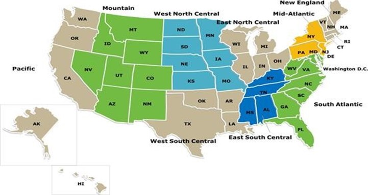
Figure 1: United States by Region. Image Source. States that are contiguous and within the same region have the same color for ease of distinguishing the regions used in analysis.

Model I included the individual- and aggregate-level sociodemographic covariates and saved the residuals for use in the subsequent model. Model II included the 12 appraisal scores to predict the covariate residuals from Model I and saved the new residuals for use in the subsequent model. Model III included the categorical variable for region to predict the residuals from Model II and saved the new residuals for use in the subsequent model. Model IV included 12 region-by-appraisal interactions to predict the Model III residuals. Due to the relatively large sample size and the many comparisons considered to test our hypotheses, we decided to focus on effect sizes that were “small” or larger using Cohen’s criteria [26] rather than on p-values. Accordingly, individual predictors’ eta-squared (η²) statistics had to be at least 0.01 (1% of variance explained) for us to consider them noteworthy. Statistical analyses were implemented using IBM SPSS version 26 [27].

Results

Individual-Level Sample Demographics
The analytic sample included between 2,853 and 3,955 people who had complete data on the relevant measures for a given analysis. This sample represented between 68% and 95% of the 4,174 respondents. In other words, due to sporadic missing data, different subsets of the 4,174 were kept in the analyses. Table 1 provides the individual-level sociodemographic characteristics. The sample was comprised mostly of patients (82%), with a mean age of 48 years, and mean age at diagnosis was 41 years. The sample was predominantly female (86%), White (91%), married or cohabitating (67%), and not currently employed (53%). While 53% of respondents had completed college or more education, only about 28% of their parents had. The median income range was $ 50,000-100,000.

Table 1: Person-Level Demographic Characteristics (N = 3,955), United States, 2016

Aggregate-Level Sample Demographics
Table 2 provides the aggregate-level sociodemographic characteristics considered in the analysis. Nine of the ten regions had sufficient sample sizes to be retained in subsequent multivariate analyses (i.e., non- contiguous states were excluded from analysis). The majority of respondents lived in a metropolitan area [22], with mean population natural log [Ln] of 9.9 (i.e., about 20,000 people in their ZIP Code) and a mean Ln density of 6.8 (i.e., about 900 people per square mile). The median household income by ZIP Code was about $60,000, and 9% of the people in the ZIP codes included in our sample were below the poverty level. The mean Gini coefficient by state was 0.47, which is mid-range in the worldwide empirical distribution of 0.24-0.63 [24,25], where zero indicates a perfectly uniform distribution of population wealth.

Table 2: Aggregate-Level Demographic Characteristics (N=3,955)

Regional Differences in Appraisal?
Table 3 show results of the MANOVA investigating the importance of region (independent variable) in predicting the 12 appraisal scores (dependent variables), after adjusting for individual- and aggregate-level sociodemographic covariates. The overall model explained nearly 34 % of the variance (sum of all partial η² = 0.339). Among the sociodemographic covariates, significant multivariate effects predicting appraisal were detected for marital status, race, income, being employed, education, mother’s education, number of comorbidities, age, age at diagnosis, and area population (data not shown). In predicting appraisal variables, all of the models had eta-squared coefficients that qualified as “small” using Cohen’s criteria. Over and above the afore mentioned sociodemographic covariates, region had a multivariate effect that was statistically significant (omnibus results for Pillai’s Trace F = 1.81, df = 96, 22,440; p < 0.0001) but practically insignificant.

Table 3: Results of MANOVA investigating regional differences in appraisal (N = 2853)

*Bolded if η2 > .020 for overall model or if partial η2 > 0.010 for region variable or for individual regions.

Appraisal scores did not differ substantially by region. After adjusting for covariates, no regional appraisal difference accounted for an η2 larger than 0.013. Even for the domain that best distinguished regions (Spiritual Focus), mean differences were so small as to be barely visible, even when regions were sorted by mean (see dotted line of the overall mean in Figure 2).

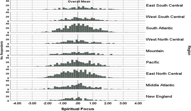
Figure 2: Spiritual Focus Means by Region

Regional Differences in Relationship between Resilience and Appraisal
As a basic indicator of the way relationships did or did not differ by region, Table 4 shows correlation coefficients between appraisal and resilience by region, with conditional formatting to indicate the effect size. Of note, Wellness Focus, Health Worries, and Recent Challenges had consistent medium or small correlations across regions with one or two exceptions by region. Relationship Focus and Maintain Roles generally had correlations less than ± 0.10, with a few exceptions that were between 0.10 and 0.30 (i.e., small effect size). The next model, with Model I residuals as a dependent variable (i.e., resilience adjusted for sociodemographic), explained 17% of the variance by including the 12 appraisal composite scores. Appraisal patterns associated with greater resilience were characterized by a greater emphasis on Wellness and Spiritual Focus, and less on Health Worries, Recent Challenges, Anticipating Decline, and Being Worry-Free (p < 0.0001 to 0.02). The next model, with Model II residuals as a dependent variable (i.e., resilience adjusted for sociodemographic and appraisal), explained just 0.1% of the variance by including Region. The final model, with Model III residuals (i.e., resilience adjusted for sociodemographic, appraisal, and region) as a dependent variable, explained even less of the variance (0.05%) by including Appraisal-by-Region interactions.

The universality we observed in the QOL appraisal-resilience connection has distinct clinical implications. It suggests ways in which cognitive- coaching interventions could help patients and caregivers increase their resilience. Our results support the kind of interventions that help individuals to pursue a calm, healthy lifestyle; practice self-acceptance; and maintain activities that help them remain positive and balanced. Our results also support de-emphasizing rumination about “worst moments.” In parallel, our results support the benefit of a “spiritual focus,” one that prioritizes helping others, leaving a legacy of a positive impact on the world, and finding ways to feel part of something greater than oneself. All these cognitive appraisal processes were distinctly associated with greater resilience in the face of health problems. While the study sample is large and heterogeneous in its illness representation, some limitations must be acknowledged. First, the data are cross-sectional, limiting our ability to make causal inference. Second, the sample disproportionately reflects some demographic characteristics (i.e., middle-aged, white, female, married, and/or living with family members), which may affect external validity. Third, some aggregate-level demographic indicators were limited by the public unavailability of more recent data. Fourth, it is possible that the listwise deletion in the MANOVA analyses (i.e., from 3,955 to 2,853 cases) biased coefficients. Fifth, our regional comparisons were limited by the available sample sizes, which reduced our power to detect small effect sizes.

Generally speaking, researchers do not like to report null results. In this case, however, our null results underscore important commonalities in appraisal, resilience, and the appraisal- resilience connection across diverse geographic regions.

They also suggest a wide applicability of relatively standardized interventions to support resilience. We did find that resilience was negatively associated with being disabled from work, having more comorbidities, and being older. Such sociodemographic factors as well as SES factors per se can present potent barriers to treatment adherence, which is increasingly the focus of attention among healthcare providers promoting person-centered healthcare [28,29]. Social-service initiatives that can help individuals with such challenges may by extension better enable clinical interventions aimed at strengthening resilience. With pragmatic solutions to such barriers, we see great promise in appraisal-based approaches to helping individuals become more resilient in the face of health challenges.

Table 4: Pearson Correlation Coefficients Summarizing Resilience-Appraisal Association by Region

Table 5. Summary of Results of Hierarchical Series of Regressions Predicting Resilience

Declarations
Ethics approval and consent to participate. The study was reviewed and approved by the New England Review Board (NEIRB#15-254), and all participants provided informed consent. All procedures performed in studies involving human participants were in accordance with the ethical standards of the institutional and/or national research committee and with the 1964 Helsinki declaration and its later amendments or comparable ethical standards.

Availability of Data and Material: The study data are confidential and thus not able to be shared.

References

1.  Padilla GV, Mishel MH, Grant MM (1992) Uncertainty, appraisal and quality oflife. Qual Life Res 1(3): 155-165. 
2. Rapkin BD, Fischer K (1992) Personal goals of older adults: issues in assessment and prediction. Psychol Aging 7(1): 127-137.
3. Rapkin BD, Schwartz CE (2004) Toward a theoretical model of quality- of-life appraisal: Implications of findings from studies of response shift. Health and qual life outcomes 2(1): 14.
4. Rapkin B, Weiss E, Chhabra R, Ryniker L, Patel S, et al. (2008)  Beyond satisfaction: Using the Dynamics of Care assessment to better understand patients' experiences in care. Health and Qual  Life Outcomes 6(1): 20.
5. Schwartz CE, Rapkin BD (2004) Reconsidering the psychometrics of quality of life assessment in light of response shift and appraisal. Health and Qual Life Outcomes 2: 16.
6. Tourangeau R, Rips LJ, Rasinski K (2000) The Psychology of Survey Response. Cambridge: Cambridge University Press.
7. Yuelin Li,Rapkin BD (2009) Classification and regression tree analysis to identify complex cognitive paths underlying quality of life response shifts : A study of individuals living with HIV/AIDS. J Clinical Epidemiol 62: 1138-1147.
8. Rapkin BD, Schwartz CE (2016) Distilling the essence of appraisal: a mixed methods study of people with multiple sclerosis. Qual Life Res 25(4): 793-805.
9. Schwartz CE, Powell VE, Rapkin BD (2017) When Global Rating of Change contradicts observed change: Examining appraisal processes underlying paradoxical responses over time. Quality of Life Research26: 847-857.
10. Taminiau-Bloem EF, Van Zuuren FJ, Visser MR, Tishelman C, Schwartz CE (2010) Opening the black box of cancer patients’ quality- of-life change assessments: a qualitative study examining the cognitive processes underlying responses to transition items. Understanding changes in in cancer patients: A cognitive interview approach:163.
11. Bochner, B, Schwartz CE, Garcia I, Goldstein L, Zhang J, et al. (2017) Understanding the impact of radical cystectomy and urinary diversion in patients with bladder cancer: treatment outcomes clarified by appraisal process. Qual Life Res 26(Suppl): 6.
12. Nunn A, Yolken A, Cutler B, Trooskin S, Wilson P, et al. (2014) Geography should not be destiny: focusing HIV/AIDS implementation research and programs on microepidemics in US neighborhoods. Am J Public Health 104(5):775-780.
13. Stopka TJ, Goulart MA, Meyers DJ, Hutcheson M, Barton K, et al. (2017) Identifying and characterizing hepatitis C virus hotspots in Massachusetts: a spatial epidemiological approach. BMC Infect Dis 17(1): 294.
14. Stopka TJ, Lutnick A, Wenger LD, Deriemer K, Geraghty EM., et al. (2012) Demographic, risk, and spatial factors associated with over-the- counter syringe purchase among injection drug users. Am J Epidemiol 176(1): 14-23.
15. Stopka TJ, Krawczyk C, Gradziel P, Geraghty EM (2014) Use of spatial epidemiology and hot spot analysis to target women eligible for prenatal women, infants, and children services. Am J Public Health 104(Suppl 1): S183-S189.
16.  Schwartz CE, Zhang J, Rapkin BD, Finkelstein JA (2019) Reconsidering the minimally important difference: evidence of instability over time and across groups. Spine J 19(4): 726-734. 
17.  Rapkin BD, Garcia I, Michael W, Zhang J, Schwartz CE (2017) Distinguishing appraisal and personality influences on quality of life in chronic illness : Introducing the Quality-of-Life Appraisal Profile version 2. Qual Life Res 26: 2815-2829.
18. Reed BR, Mungas D, Farias ST, Harvey D, Beckett L et al. (2010) Measuring cognitive reserve based on the decomposition of episodic memory variance. Brain 133: 2196-2209. 
19. Schwartz CE, Michael W, Rapkin BD (2017) Resilience to health challenges is related to different ways of thinking : Mediators of quality of life in a heterogeneous rare-disease cohort. Qual Life Res 26(11): 3075-3088.
20. Davis JA, Weber RP (1985) The logic of causal order (Vol. 55, University Paper Series on Quantitative Applications in the Social Sciences, Vol. 07-004). Newbury Park, CA: Sage.
21. US Census (2013) Factfinder.Census.gov, a 10-step. Accessed July 16, 2019.
22. Inter-university Consortium for Political and Social Research (2003) Accessed July 16, 2019.
23. American Community Survey (2010) Gini index for US as tabulated in the 2010 American Community Survey.
24. Atkinson AB (1970) On the measurement of inequality. J Economic Theory 2(3): 244-263.
25. Trapeznikova I (2019) Measuring income inequality. IZA World of Labor.
26. Cohen J (1992) A power primer. Psychological Bulletin 112: 155-159.
27. IBM (2019) IBM SPSS Statistics for Windows. (26th edition) Armonk, NY: IBMCorp.
28. Barry MJ, Edgman-Levitan S (2012) Shared decision making—The pinnacle patient- centered care.
29. Zulman DM, Haverfield MC, Shaw JG, Brown-Johnson CG, Schwartz R, et al. (2020) Practices to Foster Physician Presence and Connection with Patients in the Clinical Encounter. Jama 323(1): 70-81.  

Appendix Table A.1. Description of QOLAPv2 Appraisal Component Scores*

*Adopted with permission from Rapkin et  al., [17].                                                                 Total 57.6